This group contains seven interactive tools designed to illus- trate the time response (step response) of continuous linear time invariant (LTI) systems. An interactive tool has also been incorporated to explain the fitting of linear models from experimental data.
Time response of continuos-time first-order systems without zeros
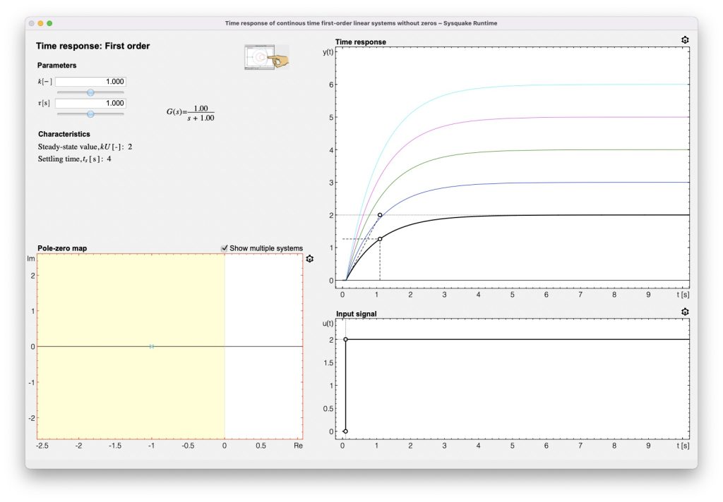

The main objective of this tool is to analyze the step response of a continuous time LTI first-order system based on the pole location and the static gain values. Thus, the relationships among the s-plane, the transfer function and the time response are analyzed. The application is fully interactive, in such a way that the modification of a parameter or a representative value in the time response is reflected automatically in the rest of the tool representations.
Time response of continuos-time second-order systems without zeros
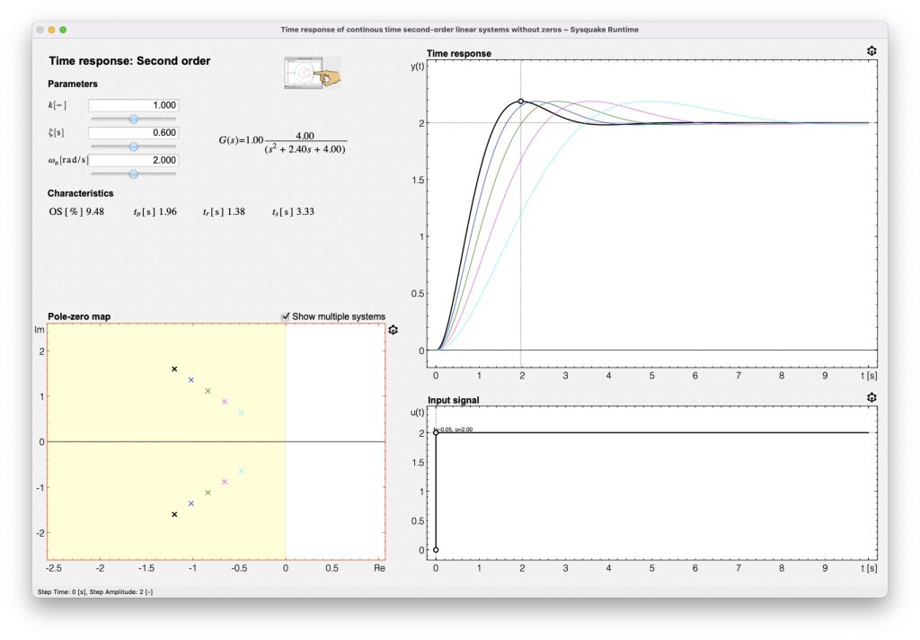
The main objective of this tool consists of analyzing the step response of continuous time second-order LTI systems based on their characteristic parameters. Comparisons between different systems can be made by setting some of their characteristic parameters ζ, ωn, σ, ωd.
Effect of a zero on the time response of continuos-time first-order systems
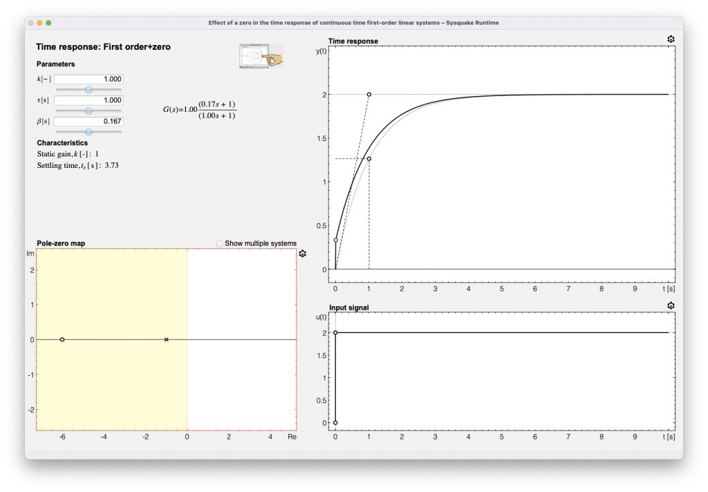
The main objective of this tool consists of analyzing the step response of a contin- uous time first-order LTI system with a zero based on its characteristic parameters. Special attention will be paid to the initial value of the step response and to understand the inverse response when the zero of the transfer function is in the right-half plane.
Effect of a zero on the time response of continuos-time second-order systems
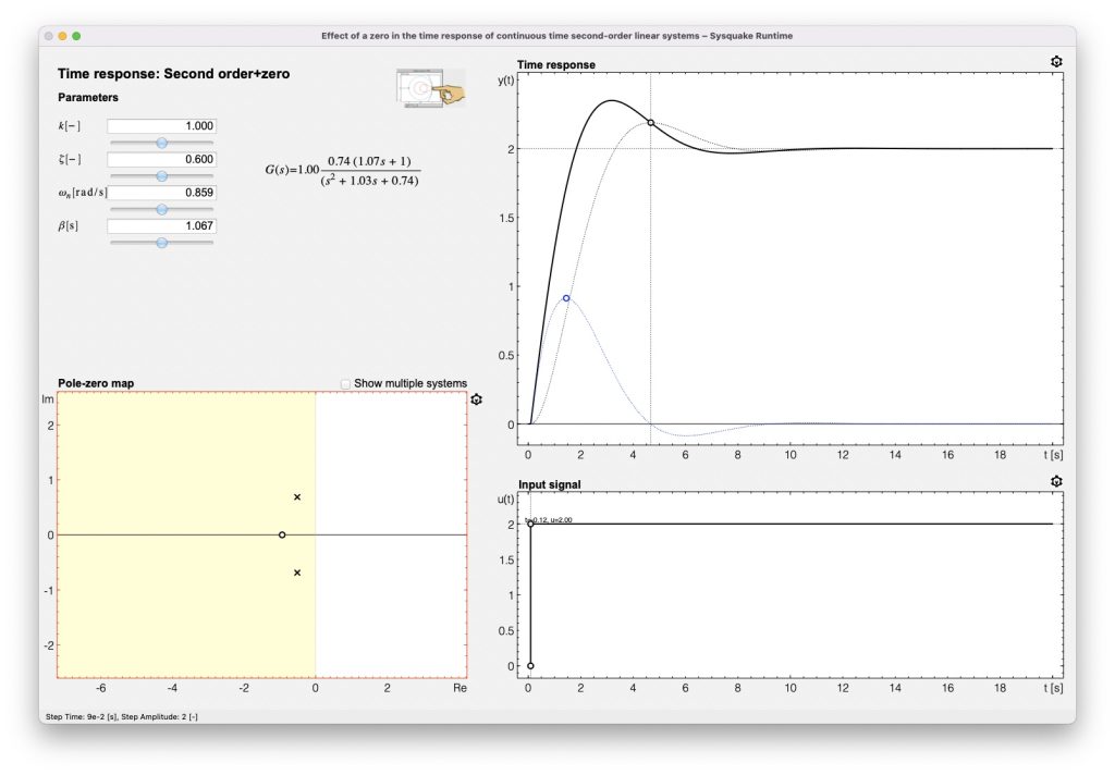
The main objective of this tool consists of studying and analyzing the effect of a zero on the time response of a continuous second-order system in an interactive way. It is very useful to analyze the inverse response concept.
Time response of generic continuos-time linear systems
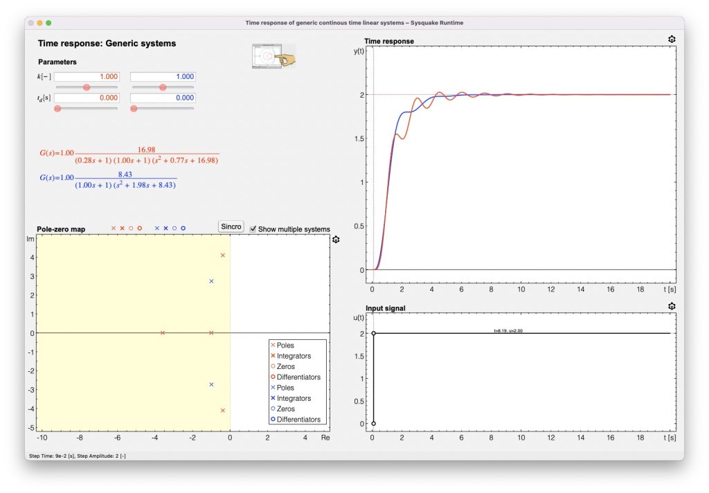
The main purpose of this tool is to analyze the time response of generic LTI systems. Generic means that the system has an arbitrary number of poles (including integrators), an arbitrary number of zeros (including differentiators) and time delay. The tool ensures that the transfer functions are causal (meaning that the denomina- tor polynomial degree must be greater than that of the numerator). A limitation on the number of poles and zeros has been included in the tool to preserve computa- tional efficiency. This tool is also useful to analyze the time response to other inputs different to steps (impulse, ramp, parabola, etc.), using the properties of linear systems and the possibility of including integrators and differentiators in the transfer functions.
Dominance in the time domain
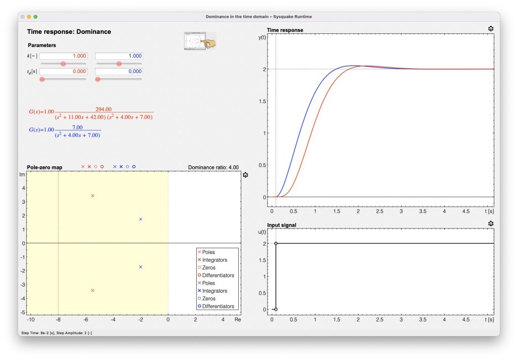
This tool deals with the dominance and dominance ratio concepts in high-order system, including representative examples. This is very useful to obtain reduced equivalent models of high-order transfer functions.
Model fitting in the time domain
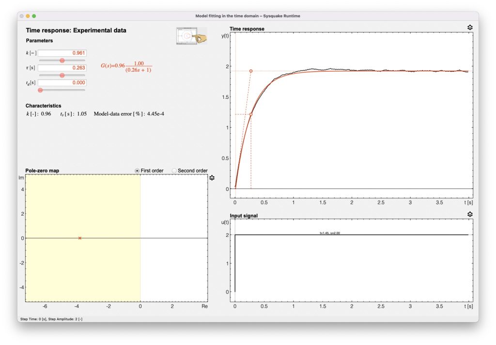
This tool is devoted to fitting experimental data to linear FODT and SODT model structures. It serves as a simple introduction to model identification to verify that low-order models can be easily calibrated using step response data, but the complexity increases as the order of the model does.